About time periods

About time periods, time points and treatment years

Heureka is using a discrete time period model, typically using five-year time intervals. The term time period is somewhat misleading, because a "time period" may refer to a time point or a period, depending on context. For example, if you use StandWise to project the growth of a stand, the "time period" is actually better interpreted as a time index marking the beginning of a period. For a case with many stands in PlanWise or RegWise on the other hand, the time index marks the midpoint of a time period. The motivation for this is that although all stands scheduled for harvest in the first period have been assigned the same treatment year (year 2.5) in the model, they should harvested simultaneously, but the harvest activities would be spread out evenly over the five-year period.

Use period midpoints if running PlanWise

When running a TPG simulation in PlanWise, period midpoints are used as default. This means that the initial state is projected 2.5 years, before the actual harvest scheduling begins. After that, five-year intervals are used. The reason for using period midpoints, is that usually some of the stands scheduled for harvesting in a certain five-year period, will not be harvested in the beginning of the period. Instead, some will be harvested early in the period, and other later in the period. Therefore, if period midpoints were not used, the harvest volumes would be underestimated.

We have no definite answer on how few or how many stands there should be to use midpoints, but if you want the results to reflect that "some time during this period these stands should be harvested", then you should use period midpoints.

Do not use period midpoints if running StandWise

In StandWise you can use period midpoints too, but it would probably make little sense expect if the purpose was to make some comparison or addition to a PlanWise simulation (for a certain stand).

Period year and treatment year

In Heureka, each period has an associated year (found in TreatmentData.Year), which refers no the number of years that has passed since the start.

Year 0: Now (start of the analysis) Year 5: Five year after the start = Beginning of the sixth year.

Note that when using period midpoints (default in PlanWise), the first period index (0) refers starting states for the analysis. In this case, the first actual planning period where optional treatments can be simulated is period 1. Period 1 has period year 2.5, i.e. the midpoint of the first five years, meaning that the period covers year 1 to 5. Period 2 covers years 6-10, and so on.

”Before” and “After” values

In Heureka, most variables has a before and after-component, which refers to the state or value before treatment, and immediately after treatment, respectively. Only before-treatment values are saved in the result database (when you run PlanWise or RegWise or save a simulation in StandWise).

State, yield and change variables

State variable

A state variable refers to a description variable for a stand at a certain time, for example the mean age or the volume.

Yield variable

A yield variable refers to some output from an activity, such as the harvest volume.

Change variable

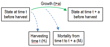
A third type of variable describes change of a stand, for example growth and mortality. Growth and mortality that are reported in a certain time period t, represents the growth and mortality that has occurred after harvesting in the previous period (t -1) to the current period year.

Basic calculation steps

As a Heureka user, it is important that you have a fundamental understanding of how a prognosis is done. The following principal steps are performed when making a prognosis from one time point (t) to another (t+1):

1. Calculate state variables for the stand at time t from tree-level data, for example stand volume and mean diameter. This is the Before-value.
2. Apply treatment, if a treatment should be applied, and update the After-value for the treatment unit. “After” is the state immediately after the treatment.
3. Calculate diameter growth, height growth and mortality for each tree.
4. Calculate ingrowth of new trees.
5. Update attributes (such as volume, age, diameter, weight) for each tree. The weight is the number of stems that a tree object represents, and is reduced by the mortality rate and by harvesting (for example a thinning will reduce the weight for one or more tree objects).
6. Let t = t + 1. Update the tree list for this period and repeat from step 1.

Subtract half a period’s harvest volume to obtain standing stock if many stands

If you want to create for example a graph of how the standing stock (the total volume) of a large forest holding develops over time according to a simulation in PlanWise, and you have used period midpoints (the default in a TPG-simulation), you should subtract half the period’s harvest volume from the Before-value. The reason is that the Before-value has been adjusted for a half a period’s growth and mortality, but not for half a periods harvesting. In reality, in a case with many stands, some of the stands will be harvested early in the period, other stands in the middle of the period, and other stand at the end of the period. But in the model, all harvesting takes place in the middle of the period. Extracting half a periods harvesting is a simple way to at least approximately adjust for this error.

Understanding how growth is calculated

Growth and mortality change refers to how a forest stand is changing from one time point to the next. Growth is reported as gross growth and net growth. Gross growth includes mortality, net growth does not.

see Growth Results